[CTU project] Self-driving robot with OpenCV

This project is done by Huỳnh Long and Nguyễn Hùng Khanh (IT cohort 40) as their graduation thesis at ICT College, Can Tho University.
Summary: This project focuses on building a self-driving robot model capable of detecting signs, traffic lights, and obstructions. To perform these functions, Haar cascade method was used to identify signs and traffic lights, then trigger the stop or continue command. Moreover, ANN was adopted to determine the movement direction (go straight, turn left, turn right) of robot from a training set of road lines' photos.
List of hardware components:

• Raspberry pi 3
• Raspberry Pi Camera
• Raspberry Pi Battery
• HC-SR04 Ultrasonic Sensor
• Robot frame
• 4 DC Motors & Wheels
• L298N motor controller

Author: Huỳnh Long, Nguyễn Hùng Khanh
Advisor: Thái Minh Tuấn, Nguyễn Ngọc Mỹ
Year: 2018.

Xem tiếp

libsvm - How to use?

libsvm is a popular library for performing Support Vector Machine algorithm. This library is developed by Chih-Chung Chang and Chih-Jen Lin, professor at National Taiwan University. Next, I will show you how to install the libsvm in MATLAB.

1. Installation

• Step 1. Download the libsvm from http://www.csie.ntu.edu.tw/~cjlin/libsvm/ and unzip it. There are some important files as in the following figure:
  
  

Xem tiếp

Useful chunks of MATLAB code for file/folder manipulation

1. Read all file names inside a range of folders

The following code will look into folders, with regarding to the folder name pattern, and read all file names inside the dedicated folder.
Example: Data files are collected from many user, and each user has it own folder with the name u001, u002,...These user folders belong to a root folder (as in the following photo).

The MATLAB code to read all data file names in this case is:

fileCfg=struct(...
            'rootFolder','D:\Experiment\BodyDyn',...
            'userFolderPattern','^u\d+$',... %regular expression for user folder names
            'extension','set'); %File extension filter
userf = dir(fileCfg.rootFolder);
userf = regexpi({userf.name},fileCfg.userFolderPattern,'match');
userf = [userf{:}];
%userf is now a row matrix that holds all user folder names

dataFiles=[];
for i=1:size(userf,2)
    temp=char(strcat(fileCfg.rootFolder,'\',userf(i),'\*.',fileCfg.extension)); %full path to data folder
    temp2 = (dir(temp)); %this will cause error if the file date is empty
    temp2 = { temp2.name };
    dataFiles=[dataFiles; temp2'];
    %dataFiles is now a vector that holds all file names
end

Important functions that you may need to understand: dir (list folder contents), regexpi (match regular expression with case insensitive).

2. Save results to file

In the following code, it will generate the file that packs the variables varX and varY. This file will be saved in the same folder of the current M file.

fileFullPath=mfilename('fullpath');
temp=strsplit(fileFullPath,'\'); %decompose the fullpath into folder parts and file name part
temp(end)=[]; %remove file name part
temp=strjoin(temp,'\'); %temp is now the path to the folder of current M file
filepath=strcat(temp, '\', datestr(now,'yyyymmdd_HHMM'), '_myData.mat');
save(char(filepath),'varX', 'varY'); %save file with timestamp
disp(['File is saved to: ' filepath]);

(Nguyen My - 2015/04/20)

Xem tiếp

A geometric interpretation of the covariance matrix

Contents

• 1 Introduction
• 2 Eigendecomposition of a covariance matrix
• 3 Covariance matrix as a linear transformation
• 4 Conclusion

Introduction

In this article, we provide an intuitive, geometric interpretation of the covariance matrix, by exploring the relation between linear transformations and the resulting data covariance. Most textbooks explain the shape of data based on the concept of covariance matrices. Instead, we take a backwards approach and explain the concept of covariance matrices based on the shape of data.
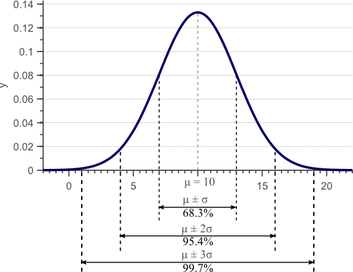
In a previous article, we discussed the concept of variance, and provided a derivation and proof of the well known formula to estimate the sample variance. Figure 1 was used in this article to show that the standard deviation, as the square root of the variance, provides a measure of how much the data is spread across the feature space.

Figure 1. Gaussian density function. For normally distributed data, 68% of the samples fall within the interval defined by the mean plus and minus the standard deviation.

We showed that an unbiased estimator of the sample variance can be obtained by:

(1)  

Xem tiếp